Map Coordinates and Land Divisions
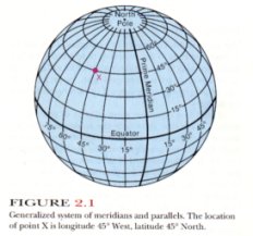
The earth’s surface is arbitrarily divided into a system of reference coordinates called latitude and longitude. This coordinate system consists of imaginary lines on the earth’s surface called parallels and meridians (fig. 2.1). Both of these are best described by assuming the earth to be represented by a globe with an axis of rotation passing through the North and South poles. Meridians are circles drawn on this globe that pass through the two poles. Meridians are labeled according to their positions, in degrees, from the zero meridian, which by international agreement passes through Greenwich near London, England. The zero meridian is commonly referred to as the Greenwich meridian. If meridional lines are drawn for each 15° in an easterly direction from Greenwich (toward Asia) and in a westerly direction from Greenwich (toward North America), a family of great circles will be created. Each one of the great circles is labeled according to the number of degrees it lies east or west of the Greenwich or zero meridian. The 180° west meridian and the 180° east meridian are one and the same great circle, and constitute the International Date Line.
A great circle represents the intersection of a plane that connects two points on the surface of a sphere and passes through the center of the sphere, in this case, the earth. The intersection of the plane with the surface divides the earth into two equal halves—hemispheres—and the arc of the great circle is the shortest distance between two points on the spherical earth.
Another great circle passing around the earth midway between the two poles is the equator. It divides the earth into the Northern and Southern Hemispheres. A family of lines drawn on the globe parallel to the equator constitute the second set of reference lines needed to locate a point on the earth accurately. These lines form circles that are called parallels of latitude, labeled according to their distances in degrees north or south of the equator. The parallel that lies halfway between the equator and the North Pole is latitude 45° North, and the North Pole itself lies at latitude 90° North.
This system of meridians and parallels thus provides a means of accurately designating the location of any point on the globe. Santa Monica, California, for example, lies at about longitude 118° 29’ West and latitude 34° 01’ North. For increased accuracy in locating a point, degrees may be subdivided into 60 subdivisions known as minutes, indicated by the notation’. Minutes may be subdivided into 60 subdivisions known as seconds, indicated by the notation”. Thus, a position description might read 64° 32’ 32” East, 44° 16’ 18” South.
Meridional lines converge toward the North or South Pole from the equator, and the length of a degree of longitude varies from 69.17 statute miles at the equator to zero at the poles. Latitudinal lines, on the other hand, are always parallel to each other. However, because the earth is not a perfect sphere but is slightly bulged at the equator, a degree of latitude varies from 68.7 statute miles at the equator to 69.4 statute miles at the poles. Thus, the area bounded by parallels and meridians is not a true rectangle. U.S.G.S. quadrangle maps are also bounded by meridians and parallels, but on the scale at which they are drawn, the convergence of the meridional lines is so slight that the maps appear to be true rectangles. The U.S.G.S. standard quadrangle maps embrace an area bounded by 7˝ minutes of longitude and 7˝ minutes of latitude. These quadrangle maps are called 7˝-minute quadrangles. Other maps published by the U.S.G.S. are 15-minute quadrangles, and a few of the older ones are 30-minute quadrangles.
Meridians always lie in a true north-south direction, and
parallels always lie in a true east-west direction. Magnetic north, however, is
the direction toward which the north-seeking end of a magnetic compass needle will point.
Because the magnetic poles are not coincident with the north and south ends of the
earth’s rotational axis, magnetic north is different from true north except on the
meridian that passes through the magnetic North Pole. The angle between true north and
magnetic north is called the magnetic declination, and is normally shown on the
lower margin of most U.S.G.S. maps for the benefit of those who use a compass in the field
to plot geological or other data on a base map (e.g., a U.S.G.S. standard quadrangle map).
Map Projection
While it is easy to draw the system of meridians and parallels on a globe, it is not possible to draw this system on a flat piece of paper (a map) without introducing some distortion. A wide variety of methods have been developed to reduce this distortion during the construction on a map. This process of constructing a map, the transferring of the meridians and parallels to a flat sheet of paper, is a geometric exercise called projection, and the resulting product is called a map projection. The map projection selected for use by the cartographer, one who draws maps, depends on the purpose of the map and the material to be presented.
The variety of map projections available include a group of projections that preserve the property of area, equal-area projections. On an equal-area, a coin placed any place on the map will cover the same area. These projections distort shape and the angular relations between meridians and parallels.
Conformable maps represent a group of projections that preserve shape but greatly distort area. Because many publications prefer to present maps that preserve shape, readers often have a mistaken impression of the relative size of the continents. An example of this is the size of Greenland, actually about the same size as Mexico, hut on a conformable map of the world it appears many times larger. There are a variety of projections that preserve angular relationships between the meridians and parallels or that, while preserving none of these properties, are compromises used for specific purposes. Most of the U.S.G.S. maps are drawn on a polyconic projection. This projection preserves neither shape nor area, but for the small area represented the distortion of both is at a minimum.
Range and Township
For purposes of locating property lines and land descriptions on legal documents, another system of coordinates is used in the United States and some parts of Canada. This system is tied into the latitude and longitude coordinate system, but functions independently of it. The basic block of this system is the section, a rectangular bloc of land one mile long and one mile wide. An area containing sections is called a township. While it was the intent of the original government land surveyors to make each section an exact square of land, many sections and townships are irregular in shape because of surveying errors and other discrepancies in laying out the network.
The north-south lines marking township boundaries are called range lines, and the east-west boundaries are called township lines. The coordinate system of numbering townships has as a reference or beginning point, the intersection of a meridian of longitude and a parallel of latitude, called principal meridian and baseline, respectively. A particular township is identified by stating its position north or south of the baseline and east or west of the principal meridian. The system of numbering township and range lines is shown in figure 2.2. The letter T along the right-hand margin of the large map stands for the word township, and the letter R stands for the word range. The notation T.3 N., R. 1 E. is read, “Township three north, Range one east.” Under this system, each township has a unique numerical designation. Several principal meridians and baselines are used in the coterminous United States, so that the township and range coordinate numbers are never very large.
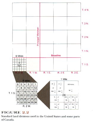
Each township consists of 36 one-square-mile sections that are numbered according to the system shown in figure 2.2. One section of land contains 640 acres.
For purposes of locating either man-made or natural features in a given section, an additional convention is employed. This consists of dividing the section into quarters called the northeast quarter (NE Ľ), the southwest quarter (SWĽ), and so on. Sections may also be divided into halves such as the north half (N˝) or west half (W˝). The quarter sections are further divided into four more quarters or two halves, depending on how refined one wants to make the description of a feature on the ground. For example, an exact description of the 40 acres of land in the extreme southeast corner of the map of section 24 in figure 2.2 would be as follows: SEĽ of the SEĽ of Section 24, T. 1 S., R. 2 W.
Topographic Maps
A topographic map is a graphic representation of the three-dimensional configuration of the earth’s surface. Most topographic maps also show land boundaries and other man-made features. The United States Geological Survey (U.S.G.S.), a unit of the Department of the Interior, has been actively engaged in the making of a series of standard topographic maps of the United States and its possessions since 1882.
Features of Topographic Maps
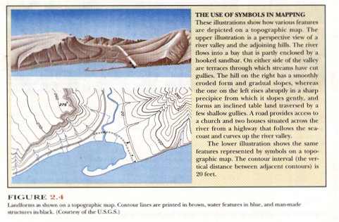
The features shown on topographic maps may be divided into
three major groups: (1) topography or relief (printed in brown), depicted by the
configuration of contour lines that show hills, valleys, mountains, plains, and the like;
(2) water features, (printed in blue), including oceans, lakes, ponds, rivers, canals,
swamps, and the like; (3) culture, (printed in black), representing manmade works such as
roads, railroads, prominent buildings, land boundaries, and similar features (fig. 2.4).
Geographical names are also printed in black.
On some topographic maps, woodland cover (forests, orchards, vineyards, and scrub) are shown in green; important roads and public land surveys in red; and where existing maps have been corrected through the use of aerial photos without field checks, the added features are shown in purple.
Standard topographic maps of the U.S.G.S. cover a quadrangle of area that is bounded by parallels of latitude (forming the northern and southern margins of the map) and by meridians of longitude (forming the eastern and western margins of the map). The published maps have different scales. A map scale is a means of showing the relationship between the size of an object or feature indicated on a map and the corresponding actual size of the same object or feature on the ground.
Geologists make use of topographic maps because they provide them with a means to observe earth features in three dimensions. Unlike other maps, topographic maps show natural features to a fair degree of accuracy in terms of length, width, and vertical height or depth. Thus by examination of a topographic map and through an understanding of the symbols shown thereon, geologists are able to interpret earth features and draw conclusions as to their origin in the light of geologic processes.
In the United States, Canada, and other English-speaking countries of the world, most maps produced to date have used the English system of measurement. That is to say, distances are measured in feet, yards, or miles; elevations are shown in feet; and water depths are recorded in feet or fathoms (1 fathom inter- 6 feet). In 1977, in accordance with national policy, the U.S.G.S. formally announced its intent to convert all of its maps to the metric system. As resources and circumstances permit, new maps published by the U.S.G.S. will show distances in kilometers and elevations in meters. The conversion from English to metric units will take many decades in the United States. In this manual, most maps used will be those published by the U.S.G.S. prior to the adoption of the metric system, because the metric maps are still insufficient in number to portray the great diversity of geologic features presented in this manual. However, some examples of map scales in metric units will be given to acquaint students with the system.
Elements of a Topographic Map
Topography
Topography is the configuration of the land surface and is shown by means of contour lines (fig. 2.4). A contour line is an imaginary line on the surface of the earth connecting points of equal elevation. The contour interval (C.I.) is the difference in elevation of any two adjacent contour lines. Elevations are given in feet or meters above mean sea level. The shore of a lake is, in effect, a contour line because every point on it is at the same level (elevation).
Contour lines are brown on the standard U.S.G.S. maps. The CI. is usually constant for a given map and may range from 5 feet for flat terrain to 50 or 100 feet for a mountainous region. C.I.’s for U.S.G.S. maps using the metric system are 1, 2, 5, 10, 20, 50, or 100 meters, depending upon the smoothness or ruggedness of the terrain to be depicted. Usually, every fifth contour line is printed in a heavier line than the others and bears the elevation of the contour above sea level. In addition to contour lines, the heights of many points on the map, such as road intersections, summits of hills, and lake levels are shown to the nearest foot or meter on the map. These are called spot elevations and are accurate to within the nearest foot or meter. More precisely located and more accurate in elevation are bench marks, points marked by brass plates permanently fixed on the ground, and by crosses and elevations, preceded by the letters BM, printed in black on the map.
Several general statements regarding contour lines follow:
1. As noted above, contour lines connect points of equal elevation.
2. Steep slopes are shown by closely spaced contour lines.
3. Gentle slopes are shown by widely spaced contour lines.
4. Contour lines do not intersect, branch, or cross. They may become merged in a vertical overhanging cliff.
5. Contour lines always close either on the map or an adjacent map sheets.
6. When contour lines cross streams they bend upstream; that is, the segment of the contour line near the stream forms a “V" with the apex pointing in an upstream direction.
7. Closed contours appearing on the map as ellipses or circles represent hills or knobs.
8. Closed contours with hachures, short lines pointing toward the
center of the closure (i.e., pointing downslope) represent closed depressions. The outer
hachured contour line has the same elevation as the lower adjacent regular contour line.
Examine figure 2.4 for the relationship of contour lines to topography. In particular,
note the difference in spacing between the contour lines that depict the steep slope on
the left side of the river and the contour lines that depict the gentle slope on the right
side of the river. Where the cliff is almost vertical in the lower left-hand corner of the
map, the contour lines are almost "stacked” one on top of the other. Note the
formation of a “V" where a contour line crosses a stream.
Map Scale
Three scales are commonly used in conjunction with topographic maps: (1) fractional, (2) graphic, and (3) verbal.
1. A fractional scale is a fixed ratio between linear
measurements on the map and corresponding distances on the ground. ft is sometimes called
the representative fraction or R.F.
Example: R.F. 1:62,500 or 1/62,500
This notation simply means that 1 unit on the map equals
62,500 of the same units on the ground. Thus, a line 1 inch long on the map represents a
horizontal distance of 62,500 inches on the ground. (Note that the numerator of the R.F.
is always 1.)
2. A graphic scale is simply a line or bar drawn on the map and
divided into units that represent ground distances.
3. A verbal scale is a convenient way of stating the
relationship of map distance to ground distance. For example, “1 inch equals 1
mile” is a verbal scale and means that 1 inch on the map equals 1 mile on the ground.
Or, “1 cm equals 1 kin” means that 1 centimeter on the map equals 1 kilometer on
the ground.
Converting from One Scale to Another
It is sometimes necessary to convert from a fractional scale
to a verbal or graphic scale, or from verbal to fractional. This involves simple problems
in arithmetic. The following are examples of some conversion problems.
Example 1. Convert an R.F. of 1:125,000 to a verbal scale in terms of
inches per mile. In other words, how many miles on the ground are represented by 1 inch on
the map?
Solution: It is best to express the R.F. as an equation in terms of what
it actually means. Thus,
1 unit on the map = 125,000 units on the ground.
We see from this basic equation that we are dealing in the same
units on the map and on the ground. Since we are interested in 1 inch on the map,
let us substitute inches for units in the above equation. It then reads:
1 inch on the map = 125,000 inches on the ground.
The left side of the equation is now complete, since we initially
wanted to know the ground distance represented by 1 inch on the map. We have yet to
resolve the right side of the equation into miles because the problem specifically called
for a ground distance in miles. Since there are 5,280 feet in a mile and 12 inches in a
foot,
5,280 x 12 = 63,360 inches in one mile.
If we divide 125,000 inches by the number of inches in a mile, we arrive at:
125,000/63,360 = 1.97 miles.
The answer to our problem is one inch ground. 1.97 miles or, for all practical purposes, 2
miles.
Example 2. On a certain map, 2.8 inches is equal to 1.06 miles on the
ground. Express this verbal scale as an R.F.
Solution: Again, it is wise to follow simple steps to avoid confusion.
We know that, by definition,
R.F. = distance on the map/distance on the ground.
Since we were given a map distance of 2.8 inches and the equivalent ground distance of
1.06 miles, it is a simple matter to substitute these in our basic equation. Thus,
R.F. = 2.8 inches on the map/1.06 miles on the ground.
It is now necessary to change the denominator of the equation to
inches because both terms in the R.F. must be expressed in the same units. Since there are
63,360 inches in 1 mile, we must multiply the denominator by that number:
1.06 x 63,360 = 67,161.6 inches.
Now our equation reads,
R.F. = 2.8 inches/67,161.6 inches.
To complete the problem, we need to express the numerator as
unity, and so the numerator must be divided by itself. In order not to change the value of
the fraction, we must also divide the denominator by the same number, 2.8. The problem
resolves itself into,
R.F. = (2.8÷ 2.8)/(67,161.6÷ 2.8) = 1/23,986 or rounded off
to 1/24,000
If you can follow these two examples and understand them
completely, you can handle any type of conversion problem.
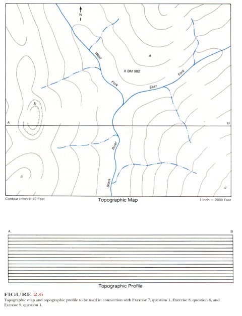
Topographic Profiles
A topographic profile is a diagram that shows the change in elevation of the land surface along any given line. It represents graphically the “skyline” as viewed from a distance. Features shown in profile are viewed along a horizontal line of sight, whereas features shown on a map or in plan view are viewed along a vertical line of sight. Topographic profiles can be constructed from a topographic map along any given line.
The vertical scale of a profile is arbitrarily selected and is usually, but not always, larger than the horizontal scale of the map from which the profile is drawn. Only when the horizontal and vertical scales are the same is the profile true, but in order to facilitate the drawing of the profile and to emphasize differences in relief, a larger vertical scale is used. Such profiles are exaggerated profiles.
Ideally both the horizontal and vertical scales would be the
same. This is impractical in most cases. On a section with a horizontal scale of
1:1,000,000, the topographic features would be almost impossible to see if the same
vertical scale were used. Both horizontal and vertical scales are usually provided with
each profile. The exaggeration is determined by comparing the inches on the profile with
feet in nature. Thus, on a profile with a horizontal scale of 1:24,000 and a vertical
scale of 1/10 inch to every 100 feet of elevation:
Horizontally 1 inch represents 24,000/12 = 2,000 ft.
Vertically 1 inch represents 10 * 100 = 1,000 ft.
Vertical exaggeration is 2.0 times.
Be aware that vertical exaggeration not only increases but also
changes the character of the profile. A volcano such as that shown in figure 2.14 would
appear as a sharp peak at 10 times vertical exaggeration.
Instructions for Drawing a Topographic Profile
1. The line along which a cross section is to be constructed may be defined by an actual line drawn on the map, or by two points on the map that determine the terminals of the line of cross section.
2. Examine the line along which the profile is to be drawn and note
the difference between the highest and lowest contours crossed by it. The difference
between them is the maximum relief of the profile. Cross sectional paper divided into 0.1
inch
or 2 mm squares makes a good base on which to draw a profile. Use a vertical scale as
small as possible so as to keep the amount of vertical exaggeration to a minimum. For
example, for a profile along which the maximum relief is less than 100 feet, a vertical
scale of 0.1 inch or 2 mm 5, 10, 20, or 25 feet is appropriate. For a profile with 100 to
500 feet of maximum relief, a vertical scale of 0.1 inch or 2 mm = 40 or 50 feet is
proper. If the maximum relief along the profile is between 500 and 1,000 feet, a vertical
scale of 0.1 inch or 2 mm = 80 or 100 feet is adequate. When the maximum relief is greater
than 1,000 feet, a vertical scale of 0.1 inch or 2 mm = 200 feet is appropriate. The
general rule for guidance in the selection of a vertical scale is: the greater the maximum
relief, the smaller the scale. Label the horizontal lines of the profile grid with
appropriate elevations from the contours crossed by the line of the profile. Every other
line on a 0.1 inch or 2 mm grid is sufficient.
3. Place the edge of the cross sectional paper along the line of profile. Opposite each intersection of a contour line with the line of profile, mark a short dash at the edge of the cross sectional paper. If the contour lines are closely spaced, only the heavy or index contours need to be marked. Also mark the positions of streams, lakes, hilltops, and significant cultural features on the line of profile. At the edge the of the paper, label the elevation of each dash.
4. Drop these elevations perpendicularly to the corresponding elevations represented by the horizontal lines on the cross sectional paper.
5. Connect these points by a smooth line and label significant features such as streams and summits of hills. Add the horizontal scale and write a title on the profile.